Centering Resonance Analysis¶

CRA is a network-based method for the untrained classification of documents and entire corpora, which was proposed bei Corman et al. in their 2002 article „Studying Complex Discursive System“. It is inspired by linguistic ideas about the textual „centers“, i.e. the words (mostly nouns) who contribute the most to the specific meaning of the text. To find those centers they apply structural network measures, which allow for the identification of the most central noun phrases in a text. The „resonance“ of a text is therefore defined as the measure of similarity between two texts in terms of their respective centers.

Python provides two packages, which make the implementation of this method pretty straightforward. The NLTK-Package (Natural Language Toolkit) provides realtively fast methods to deal with the linguistical side of things. Most importantly, algorithms for part-of-speech tagging, which are necessary to identify the central noun phrases of the text. The second important package is NetworkX. It implements a powerful network class as well as algorithms to analyse those networks in terms of centrality.

Corman et al. describe their method as a four-step process, which consists of selection, indexing, linking and the application of this model. Putting the actual apllication last, serves as a reminder that theoretical and methodological issues are to be considered on each step. Since our focus here lies on implementation instead of interpretation we do discuss some of these issues but are generally more concerned with showing how to apply this method using python. We use a portion of the Reuters Newswire Corpus which comes with NLTK and consists of roughly 10.000 short news for illustration.

Selection¶

In the selection stage, the corpus is reduced to its noun phrases:

CRA parses an utterance into its component noun phrases. A noun phrase is a noun plus zero or more additional nouns and/or adjectives, which serves as the subject or object of a sentence. Determiners (the, an, a, etc.), which can also be parts of noun phrases, are dropped in CRA analyses. Thus, a noun phrase is represented by one or more words, and a sentence can consist of one or more noun phrases. (Corman et al. 2002:174)

This makes it necessary to find the right part-of-speech tag for each word in the corpus. Unfortunately, the Reuters News Corpus does not come with already tagged words. Instead a POS-Tager is needed to identify nouns and adjectives. NLTK provides the Penn Treebank Tagger for these tasks. Before the tagging itself stopwords should be removed from the text because they carry very little semantic information and the reduction of the text makes computing the pos-tags much easier. Additionally only a portion of the Reuters corpus (the first 1000 documents) will be used, since both the pos tagging as well as the network analytics can become very computationally expensive.
Furthermore, the selection step as well as linking (i.e. network construction) need to be wrapped in a function definition, to preserve the ability to differentiate the documents according to the fileids or categories. This function will be introduced after a short exemplary look at one document and the single steps leading up to the network construction stage.

Using the Penn-Treebank Tagger on the sentences is rather straightforward:

Using the tagger results in a list-of-tuples, where the first entry gives us the word and the second one contains the part-of-speech tag. NLTK provides a help function (nltk.help.upenn_tagset(tagpatter)) which supports regular expressions to look up the meaning of the pos-tags. Since we are only interested in nouns and adjectives, we only take a look at them.

We can now tag all sentences in the corpus and extract their compound noun phrases.

Network Construction (Linking)¶

During this step the network is constructed from the co-occurrence of adjectives and nouns within the same sentence.

To begin with, all words comprising the centers in the utterance are linked sequentially. In the majority of cases, where noun phrases contain one or two words, the sequential connections capture all the linkage intended by the author because no higher-order connections are possible without crossing the boundaries of the noun phrases. However, there are cases where three or more words are contained in a single noun phrase. In that case, the sequential links do not exhaust the connectedness possible in the set created by the author. Hence, we link all possible pairs of words within the noun phrases. For example, the phrase “complex discursive system” would generate the links: complex-discursive, discursive-system, and complex-system. (Corman et al. 2002: 176)

In Python we can realize this with the itertools-module, This module provides methods for iterator construction, meaning a fast way to generate combinations without repetitions from a given input sequence.

The result is a list of tuples which contain the edges of the textual centers. These edges can now be made into a network by simply initialising them as a NetworkX Graph class.

Finding the Linguistic Centers (Indexing)¶

The next step in Centering Resonance Analysis uses structural network measures to characterise and analyse the content of the texts. To find the most central words within the network Corman et al. propose the usage of the betweenness centrality measure.

The result of the NetworkX algorithm is a dictionary with the nouns and adjectives as key. We can then take a look at the ranking of the words according to their betweenness centrality. Because Python dictionaries cannot be sorted itself we have to transfer them to a list-of-tuples which then can be sorted.

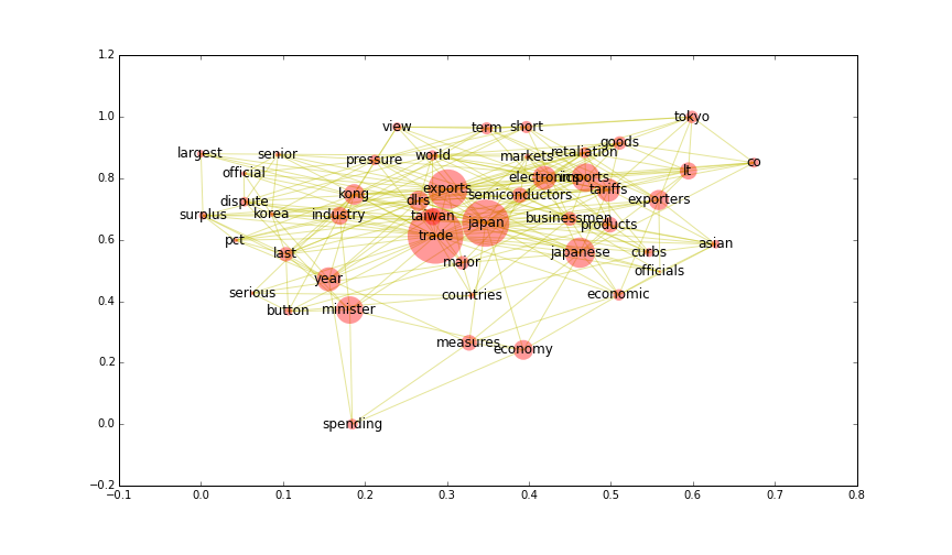
The resulting network can easily be plotted:

As mentioned earlier, the steps leading up to the construction of the network can be generalized into a single function.

The first function takes a document consisting of a list of sentences, whereby each sentence is itself a list of word tokens. In keeping with the example the tag keyword argument defaults to adjectives and nouns. This can easily be changed via regular expressions. The second function utilizes the networkx class to a greater extent, by including the betweenness centrality as a node attribute and the frequency of every edge as an attribute of that edge. This will be useful in later steps of the analysis, because it allows us to store the constructed networks more easily and keep informations, which would otherwise be lost in the transformation process.

Saving the resulting graph as a file including all its attributes can be done via the many read_ and write_ functions supplied by NetworkX. For example as a GEXF file (write_gexf()) which is essentially a modified XML representation of the graph and can be understood by a wide range of other network analysis tools.

Computing the Resonance¶

Last but not least we need a way to compute the resonance, which is a similarity measure based on comparing the different texts according to their respective centers. Corman et al. 2002 present two ways to calculate the resonance between texts. We start by looking at the simple way first, which claims to be espescially suited for broader comparisons:

The more two texts frequently use the same words in influential positions, the more word resonance they have. The more word resonance they have, the more the communicators used the same words, and the more those words were prominent in structuring the text’s coherence. Word resonance is a more general measure of the mutual relevance of two texts, and has applications in the modeling of large corpora. (Corman et al. 2002:178)

They give the following formula:

\begin{equation*} WR_{AB} = \sum_{i=1}^{N(A)} \sum_{j=1}^{N(B)} I_i^A \cdot I_j^B \cdot \alpha_{ij}^{AB} \end{equation*}

Where \(I_i^A\) represents the betweenness centrality of the \(i\)-th word in text \(A\). \(I_j^B\) is the same for text \(B\) and \(\alpha_{ij}^{AB}\) is a indicator function, which is \(0\) if the \(i\)-th word of text \(A\) and the corresponding word of the same rank in text \(B\) are not the same. If they are the same, \(\alpha\) becomes \(1\). Therefore only words with the same rank are compared.

To give an example, we need to create at least two centered network graphs to compare. These graphs do not necessarily need to be constraint to one specific document in the corpus. Instead we could treat larger (or smaller) collections of text as a single unit of analysis. When the chosen text is too small, chances are there will be a resonance of zero because there are too few similarities in the used words. Yet one has to keep in mind, that calculating the betweenness centrality of all noun phrases can become very computational expensive. For illustration purposes and the sake of simplicity a subset of the reuters corpus is chosen. The categories in the Reuters News Corpus are categorized according to economic goods and services which are mentioned in them. It therefore seems worthwhile to compare the different linguistic centers according to those economic categories. To keep it manageable, just two economic areas are chosen, namely „Finance“ and „Food“. Also, since the methods tends to become computationally expensive when confronted with larger corpora, only a subsample of the categories is used.

• Finance: „income“,“trade“, „money-supply“
• Food: „wheat“, „coffee“, „rice“, „sugar“

The function cra_centered_graph() was used, because the time it took to create the graphs and calculate the measurements made it seem reasonable to save the data before calculating the resonance. From the resulting networks we can calculate the simple, unstandardized measure of resonance. But since the data is now part of the graph object, we need to retrieve it first and transform it into a tuple. This is made easy by the get_node_attributes() function which returns a Python dictionary of the chosen attribute for a given graph.

As Corman et al. note:

This measure is unstandardized in the sense that resonance will increase naturally as the two texts become longer in length and contain more common words. There are cases, however, where a standardized measure is more appropriate. For example, in positioning documents relative to one another (as described below), one does not necessarily want to overemphasize differences in document length, number of words, and so on. (Corman et al. 2002:178)

They therefore propose a standardized measure of resonance:

\begin{equation*} WR’_{AB} = WR_{AB} / \sqrt{ \sum_{i=1}^{N(A)} (I_i^A)^2 \cdot \sum_{j=1}^{N(B)} (I_j^B)^2 } \end{equation*}

Which transfered to Python code looks something like this:

As we can now see the standardized resonance lies between 0, which means two texts have no structural similarity regarding their centers and 1 meaning they are essentially the same (which they are in this example).

The second way to compare texts is their pair resonance. This measure uses co-occuring word pairs for its comparison, while the simple resonance score is computed on the basis of co-occuring words. For this we have to calculate the influence score of every word-pair weighted by the frequency with which it occurs in a given text:

\begin{equation*} P_{ij}^T = I_i^T \cdot I_j^T \cdot F_{ij}^T \end{equation*}

The influence score of the pairing of the \(i\)-th and \(j\)-th word in a text \(T\) is given by the product of there respective influence scores \(I\) times the frequency \(F\) of there co-occurence. The pair resonance \(PR_{AB}\) between to texts is then given by the following formula:

\begin{equation*} PR_{AB} = \sum_{i=1}^{N(A)-1} \left( \sum_{j=i+1}^{N(A)} \left( \sum_{k=1}^{N(B)-1} \left( \sum_{l=k+1}^{N(B)}\left[ P_{ij}^A \cdot P_{kl}^B \cdot \beta_{ijkl}^{AB} \right] \right) \right) \right) \end{equation*}

wherein \(\beta\) is a indicator function similar to \(\alpha\) in the case of the simple resonance. It is 1 if the word-pair exists in both text and 0 otherwise.

Since we have constructed the above network as a simple, undirected graph it contains no information on the frequency of specific word pairs, because the nx.Graph() class does not allow multiple edges between the same nodes. We could have used an nx.MultiGraph() instead. However many algorithms for the calculation of network measures are not well defined on graphs with multiple edges. Such is the case for the shortest path and therefore the betweenness centrality. There are basically two ways this problem can be solved. Because we stored the frequency of the edges already as an edge attribute we can easily retrieve this information and calculate the influence score for every word-pair (\(P_{ij}^T\)) from it. This can be done by calling the nx.get_edge_attributes() function on the graph and supplying it with the name of the attribute in question. This will return a dictionary whose keys are the tuples representing the graphs edges. .

In keeping with the general theme the influence scores can also be stored as graph attributes once they are derived. Making it much easier doing other calculations later on. Therefore the next function assumes a „centered“ graph with a frequency and betweenness attribute.

Given the pair influence scores in the form of dictionaries of edges, the pair resonance can be computed like this:

As with the simple resonance score, there also exists a standardized version of the pair resonance. It is given by the formula:

\begin{equation*} {PR‘}_{AB} = PR_{AB} / \sqrt{\sum_{i=1}^{N(A)-1} \sum_{j=i+1}^{N(A)} (P_{ij}^A)^2 } \cdot \sqrt{\sum_{k=1}^{N(B)-1} \sum_{l=k+1}^{N(B)} (P_{kl}^B)^2 } \end{equation*}

As a function:

Which leaves us with the following pair resonance in our example:

Application (and Discussion)¶

The very low standardized resonance scores (simple as well as pairwise) suggest both corpora differ widely in the centers which describe them best. This notion is confirmed, when we take a closer look at the top 10 (ranked by their pair resonance scores) of noun phrases which make up those centers:

One of the first things that can be noticed here is the strong influence of noun phrases which seem to be essentially „self loops“ in the network, i.e. an edge connecting to the same node from which it originated. These edges are no artifacts, but stem from the fact that the sentences in the Reuters News Corpus are defined as ending with a colon. Therefore subordinate clauses and sentences ending in semicolons are considered to be part of the overall sentence. This can be corrected by dropping all self loops from the network or tokenizing the text differently. Yet both methods lose some information about the text and depend strongly on the information one wants to retrieve from the corpora. Since self loops are an attribute of the edges of a network, they do not interfere with the betweenness centrality of a node. Therefore their influence on the resonance scores seems to be negligble in most cases. However if two texts were written in a very particular style, where for example one would use lots of subordinate clauses and long winded sentences and the other would be very concise and use only very short sentences the error could become very pronounced. This serves as a reminder to be careful in the application of computational methods of text analysis. A lot depends on ones understanding of the internal structure of the documents in question as well as ones own research interest.

Since the texts used here served only the purpose of illustrating the method, a more extensive interpretation of the findings in terms of the resonance scores or the networks properties would require more data and preferably a solid research question. Therefore we leave the discussion of the specific properties of those networks and instead discuss the method itself.

To discuss the merits of their approach Corman et al. differentiate between three goals of computational text analysis: inference, positioning and representation. Inference refers to the idea of modelling the text according to the statistical properties it has and thus deriving informed guesses on unknown properties, i.e. text classification. For example Naive Bayes Classification or similar (un-)supervised machine learning algorithms. Corman et al. criticise those approaches for their narrow domain of application. Since they must be trained on corpora with known properties they cannot easily be transfered to documents coming from a different context. Furthermore, the authors see a lack of linguistic and semiotic background in the case of the inference models. The second approach tries to position documents in relation to other documents, by placing them in a common semantic space. Prime examples would be LSA or LDA. According to Corman et al. the problem here is the reduction of the text to a vector within the semantic space, whose position depends very much on the quality of the spatial construction and is also only defined in terms of a narrow domain. It also becomes clear that the authors see the loss of information by reducing the documents to vectors as deeply problematic. Finally, they discuss representational techniques which try to preserve most of the linguistic structure of the text. Yet these techniques can also be problematic, which leads them to propose three criteria for a „good“ representational approach:

In particular, we see a need for a representational method that meets three criteria. First, it should be based on a network representation of associated words to take advantage of the rich and complex data structure offered by that form. Second, it should represent intentional, discursive acts of competent authors and speakers. Units of analysis and rules for linking words should be theoretically grounded in discursive acts. Third, it should be versatile and transportable across contexts. Making text representations independent of dictionaries, corpora, or collections of other texts would provide researchers maximum flexibility in analyzing and comparing different groups, people, time periods, and contexts. (Corman et al. 2002:172)

The Centering Resonance Analysis seems to meet those three criteria rather well. The network representation makes it indeed easy to use different methods to analyse the structure of text. For example, instead of the betweenness centrality other measures could have been used to index the network nodes. Yet choosing between different measures and analytical technique seems problematic, for the very same reason Corman et al. had in criticising inference and positional approaches. There is no linguistic or semiotic theory which would make it possible to map the properties of the text to the network in a way that would allow for a clear interpretation of the structural properties of the network. This problem stems mostly from the fact that the network representation assumes specific tokens to be fixed nodes whose edges are constructed via co-occurences in a fixed context. This makes it hard to distinguish between different contextual usages of the same tokens. Therefore synonyms and polynyms can be considered more problematic for the representational methods than for the positional ones. We also know, that words can have very different meanings and informational values depending on the sentence they are placed in as well as the rest of the document and even in relation to the entire corpus. This is the main reason for the use of weighting schemes in topic modelling, e.g. TFIDF which weighs the distribution of words according to local as well as global parameters. Because CRA also assumes the same weight for all tokens as part of a given context, all edges are considered essentially the same across all documents with the exception of their frequency.

The second point they make is the accurate representation of discursive acts in form of a graph consisting of the central noun phrases of a given text. And while this is clearly the main strength of this method it comes at somewhat high computational costs. Finding the correct part-of-speech tags can take quite some time and generally depends on the availability of a high quality pos-tagger for this specific language. It should also be noted, that the representation of linguistic centers is only one of many discoursive acts and construction principles which play a role in the production of documents, albeit a very important one. Other discoursive acts include for example the ordering of sentences according to their priority in an argument or the represenatation of a temporal process. These are commonly reffered to as the narrative structure.

The appeal of a flexible data structure which allows for an easy exchange and cooperation among researchers without the need to transfer the entire corpus, as mentioned in the third criteria, is not lost on the author. This was basically the main reason for implementing the CRA on top of the networkx graph class. As mentioned before, this make it easy to store the data as one coherent data structure as well as expanding upon the analysis. Using inheritance and other more advanced object oriented programming techniques would have made this integration even more rewarding. Yet those techniques are beyond the capabilities of the author and would have had required much more programming knowledge from the reader. It should also be noted, that for didactic reasons this code is more geared towards readability than performance. Using sparse arrays instead of lists would result in a substantial increase of speed for the calculation of the resonance measures. However, since the real bottleneck is the pos-tagging and the calculation of the betweenness centrality, the gain in computational speed seems to be negligible.